GNUPLOT-3.7 demo: surface1.dem

#
# $Id: surface1.dem,v 1.5 1995/04/21 12:49:06 drd Exp $
#

set samples 21
set isosample 11
set xlabel "X axis" -3,-2
set ylabel "Y axis" 3,-2
set zlabel "Z axis" -5
set title "3D gnuplot demo"
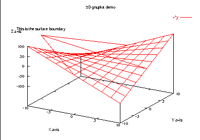
set label 1 "This is the surface boundary" at -10,-5,150 center
set arrow 1 from -10,-5,120 to -10,0,0 nohead
set arrow 2 from -10,-5,120 to 10,0,0 nohead
set arrow 3 from -10,-5,120 to 0,10,0 nohead
set arrow 4 from -10,-5,120 to 0,-10,0 nohead
set xrange [-10:10]
set yrange [-10:10]
splot x*y

pause -1 "Hit return to continue (1)"

set noarrow
set nolabel
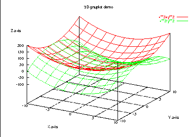
set grid
splot x**2+y**2, x**2-y**2

pause -1 "Hit return to continue (2)"

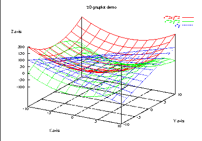
rep x*y

pause -1 "Hit return to continue (3)"

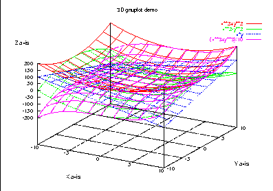
rep (x**3+y**3)/10

pause -1 "Hit return to continue (4)"

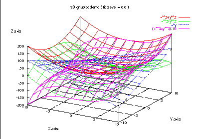
set ticslevel 0.0
set title "3D gnuplot demo ( ticslevel = 0.0 )"
rep

pause -1 "Hit return to continue (5)"

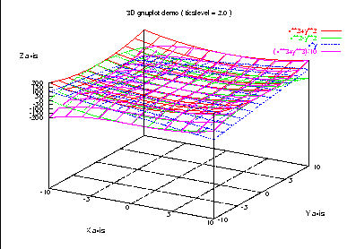
set ticslevel 2.0
set title "3D gnuplot demo ( ticslevel = 2.0 )"
rep

pause -1 "Hit return to continue (6)"

set ticslevel 0.5
set title "3D gnuplot demo ( ticslevel = 0.5 )"
rep

pause -1 "Hit return to continue (7)"

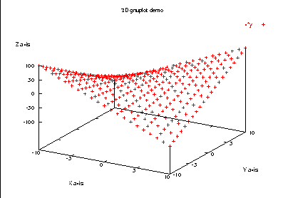
set title "3D gnuplot demo"
set nogrid
splot x*y with points

pause -1 "Hit return to continue (8)"

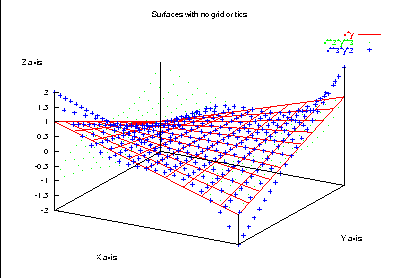
set noxtics
set noytics
set xrange [-1:1]
set yrange [-1:1]
set title "Surfaces with no grid or tics"
splot x*y with lines, x**2*y**3 with dots, x**3*y*2 with points

pause -1 "Hit return to continue (9)"

set xtics ("low" -3, "mid" 0, "high" 3)
set ytics -2,0.5,2
set xrange [-3:3]
set yrange [-3:3]
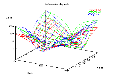
set log z
set title "Surfaces with z log scale"
splot x**2*y**2 + 2, x**2*y**4 + 2, x**4*y**2 + 2

pause -1 "Hit return to continue (10)"

set nolog z
set xtics autofreq
set ytics autofreq
set xrange [-1:1]
set yrange [-1:1]
set samples 51
set isosample 21
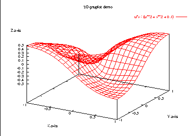
set dummy u,v
set title "3D gnuplot demo"
splot u*v / (u**2 + v**2 + 0.1)

pause -1 "Hit return to continue (11)"

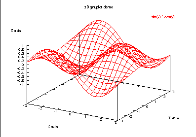
splot [x=-3:3] [y=-3:3] sin(x) * cos(y)

pause -1 "Hit return to continue (12)"

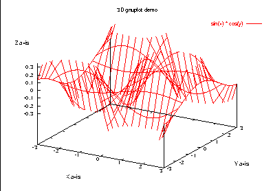
set zrange [-0.35:0.35]
replot

pause -1 "Hit return to continue (13)"

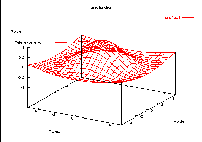
set title "Sinc function"
set zrange [-1:1]
set label 1 "This is equal to 1" at -5,-2,0.75 right
set arrow 1 from -5,-2.1,0.75 to 0,0,1
sinc(u,v) = sin(sqrt(u**2+v**2)) / sqrt(u**2+v**2)
splot [-5:5.01] [-5:5.01] sinc(u,v)

pause -1 "Hit return to continue (14)"

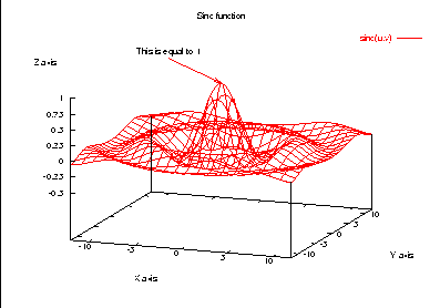
set view 70,20,1
set zrange [-0.5:1.0]
set ztics -1,0.25,1
set label 1 "This is equal to 1" at -5,-2,1.5 centre
set arrow 1 from -5,-2.1,1.4 to 0,0,1
splot [-12:12.01] [-12:12.01] sinc(u,v)

pause -1 "Hit return to continue (15)"

set noarrow
set ztics autofreq
set nolabel
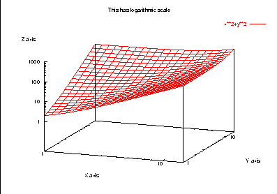
set log
set auto
set title "This has logarithmic scale"
splot [x=1:15] [y=1:15] x**2+y**2

pause -1 "Hit return to continue (16)"
set nolog
set xrange [0:15]
set yrange [0:15]
set auto
#set zrange [-0.6:0.7]

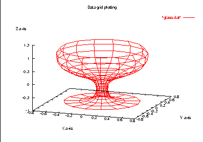
set ticslevel 0
set data style lines
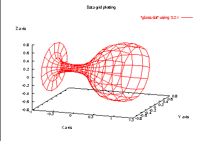
set title "Data grid plotting"
set parametric
splot "glass.dat"

pause -1 "Hit return to continue (17)"

splot "glass.dat" using 3:2:1

pause -1 "Hit return to continue (18)"

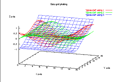
set zrange [-1.2:1.2]
set ticslevel 0.5
set noparametric
splot "glass.dat" using 1, "glass.dat" using 2, "glass.dat" using 3

pause -1 "Hit return to continue (19)"

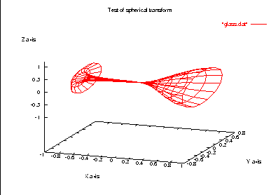
set param
set title "Test of spherical transform"
set mapp sphe
splot "glass.dat"

pause -1 "Hit return to continue (20)"

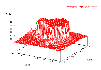
# mandelbrot demo

set nopar
set mapp cart
set view 60,30,1,1
set auto
set title "" 0,0
set isosamples 60
set hidden3d
compl(a,b)=a*{1,0}+b*{0,1}
mand(z,a,n) = n<=0 || abs(z)>100 ? 1:mand(z*z+a,a,n-1)+1
splot [-2:1][-1.5:1.5] mand({0,0},compl(x,y),30)     

pause -1 "Hit return to continue (21)"
# TANAKA Masaki  (Tokyo Institute of technology)
#                 masaki@isea.is.titech.ac.jp

#
# Clean up:
#
set samples 100
set isosamples 10
set xrange [-10:10]
set yrange [-10:10]
set zrange [-10:10]
set auto
set xlabel "" 0,0
set ylabel "" 0,0
set zlabel "" 0,0
set nohidden